72. 编辑距离
难度困难804收藏分享切换为英文关注反馈
给你两个单词 word1 和 word2*,请你计算出将 *word1 转换成 word2 所使用的最少操作数 。
你可以对一个单词进行如下三种操作:
- 插入一个字符
- 删除一个字符
- 替换一个字符
示例 1:
1 | 输入:word1 = "horse", word2 = "ros" |
示例 2:
1 | 输入:word1 = "intention", word2 = "execution" |
1 | 动态规划 |
1 | //dp solution |
132. 分割回文串 II
难度困难130收藏分享切换为英文关注反馈
给定一个字符串 s,将 s 分割成一些子串,使每个子串都是回文串。
返回符合要求的最少分割次数。
示例:
1 | 输入: "aab" |
1 | class Solution { |
5. 最长回文子串
难度中等2038收藏分享切换为英文关注反馈
给定一个字符串 s,找到 s 中最长的回文子串。你可以假设 s 的最大长度为 1000。
示例 1:
1 | 输入: "babad" |
示例 2:
1 | 输入: "cbbd" |
1 | class Solution { |
198. 打家劫舍
你是一个专业的小偷,计划偷窃沿街的房屋。每间房内都藏有一定的现金,影响你偷窃的唯一制约因素就是相邻的房屋装有相互连通的防盗系统,如果两间相邻的房屋在同一晚上被小偷闯入,系统会自动报警。
给定一个代表每个房屋存放金额的非负整数数组,计算你在不触动警报装置的情况下,能够偷窃到的最高金额。
示例 1:
1 | 输入: [1,2,3,1] |
示例 2:
1 | 输入: [2,7,9,3,1] |
1 | class Solution { |
Algorithm
It could be overwhelming thinking of all possibilities on which houses to rob.
A natural way to approach this problem is to work on the simplest case first.
Let us denote that:
f(k) = Largest amount that you can rob from the first k houses.
Ai = Amount of money at the ith house.
Let us look at the case n = 1, clearly f(1) = A1.
Now, let us look at n = 2, which f(2) = max(A1, A2).
For n = 3, you have basically the following two options:
- Rob the third house, and add its amount to the first house’s amount.
- Do not rob the third house, and stick with the maximum amount of the first two houses.
Clearly, you would want to choose the larger of the two options at each step.
Therefore, we could summarize the formula as following:
f(k) = max(f(k – 2) + Ak, f(k – 1))
We choose the base case as f(–1) = f(0) = 0, which will greatly simplify our code as you can see.
The answer will be calculated as f(n). We could use an array to store and calculate the result, but since at each step you only need the previous two maximum values, two variables are suffice.
1 | public int rob(int[] num) { |
Complexity analysis
- Time complexity : O(n)O(n). Assume that nn is the number of houses, the time complexity is O(n)O(n).
- Space complexity : O(1)O(1).
213. 打家劫舍 II
难度中等254收藏分享切换为英文关注反馈
你是一个专业的小偷,计划偷窃沿街的房屋,每间房内都藏有一定的现金。这个地方所有的房屋都围成一圈,这意味着第一个房屋和最后一个房屋是紧挨着的。同时,相邻的房屋装有相互连通的防盗系统,如果两间相邻的房屋在同一晚上被小偷闯入,系统会自动报警。
给定一个代表每个房屋存放金额的非负整数数组,计算你在不触动警报装置的情况下,能够偷窃到的最高金额。
示例 1:
1 | 输入: [2,3,2] |
示例 2:
1 | 输入: [1,2,3,1] |
1 | class Solution { |
1 | class Solution { |
Since this question is a follow-up to House Robber, we can assume we already have a way to solve the simpler question, i.e. given a 1 row of house, we know how to rob them. So we already have such a helper function. We modify it a bit to rob a given range of houses.
1 | private int rob(int[] num, int lo, int hi) { |
Now the question is how to rob a circular row of houses. It is a bit complicated to solve like the simpler question. It is because in the simpler question whether to rob num[lo] is entirely our choice. But, it is now constrained by whether num[hi] is robbed.
However, since we already have a nice solution to the simpler problem. We do not want to throw it away. Then, it becomes how can we reduce this problem to the simpler one. Actually, extending from the logic that if house i is not robbed, then you are free to choose whether to rob house i + 1, you can break the circle by assuming a house is not robbed.
For example, 1 -> 2 -> 3 -> 1 becomes 2 -> 3 if 1 is not robbed.
Since every house is either robbed or not robbed and at least half of the houses are not robbed, the solution is simply the larger of two cases with consecutive houses, i.e. house i not robbed, break the circle, solve it, or house i + 1 not robbed. Hence, the following solution. I chose i = n and i + 1 = 0 for simpler coding. But, you can choose whichever two consecutive ones.
1 | public int rob(int[] nums) { |
221. 最大正方形
难度中等403收藏分享切换为英文关注反馈
在一个由 0 和 1 组成的二维矩阵内,找到只包含 1 的最大正方形,并返回其面积。
示例:
1 | 输入: |
1 | class Solution { |
Approach #1 Brute Force [Accepted]
The simplest approach consists of trying to find out every possible square of 1’s that can be formed from within the matrix. The question now is – how to go for it?
We use a variable to contain the size of the largest square found so far and another variable to store the size of the current, both initialized to 0. Starting from the left uppermost point in the matrix, we search for a 1. No operation needs to be done for a 0. Whenever a 1 is found, we try to find out the largest square that can be formed including that 1. For this, we move diagonally (right and downwards), i.e. we increment the row index and column index temporarily and then check whether all the elements of that row and column are 1 or not. If all the elements happen to be 1, we move diagonally further as previously. If even one element turns out to be 0, we stop this diagonal movement and update the size of the largest square. Now we, continue the traversal of the matrix from the element next to the initial 1 found, till all the elements of the matrix have been traversed.
Java
1 | public class Solution { |
Complexity Analysis
- Time complexity : O((mn))O((m**n)2). In worst case, we need to traverse the complete matrix for every 1.
- Space complexity : O(1)O(1). No extra space is used.
Approach #2 (Dynamic Programming) [Accepted]
Algorithm
We will explain this approach with the help of an example.
1 | 0 1 1 1 0 |
We initialize another matrix (dp) with the same dimensions as the original one initialized with all 0’s.
dp(i,j) represents the side length of the maximum square whose bottom right corner is the cell with index (i,j) in the original matrix.
Starting from index (0,0), for every 1 found in the original matrix, we update the value of the current element as
dp(i,j)=min(dp(i−1,j),dp(i−1,j−1),dp(i,j−1))+1.dp(i,j)=min(dp(i−1,j),dp(i−1,j−1),dp(i,j−1))+1.
We also remember the size of the largest square found so far. In this way, we traverse the original matrix once and find out the required maximum size. This gives the side length of the square (say maxsqlenmaxsqle**n). The required result is the area maxsqlen2m*axsqlen*2.
To understand how this solution works, see the figure below.

An entry 2 at (1,3)(1,3) implies that we have a square of side 2 up to that index in the original matrix. Similarly, a 2 at (1,2)(1,2) and (2,2)(2,2)implies that a square of side 2 exists up to that index in the original matrix. Now to make a square of side 3, only a single entry of 1 is pending at (2,3)(2,3). So, we enter a 3 corresponding to that position in the dp array.
Now consider the case for the index (3,4)(3,4). Here, the entries at index (3,3)(3,3) and (2,3)(2,3) imply that a square of side 3 is possible up to their indices. But, the entry 1 at index (2,4)(2,4) indicates that a square of side 1 only can be formed up to its index. Therefore, while making an entry at the index (3,4)(3,4), this element obstructs the formation of a square having a side larger than 2. Thus, the maximum sized square that can be formed up to this index is of size 2×22×2.
Java
1 | public class Solution { |
Complexity Analysis
- Time complexity : O(mn)O(m**n). Single pass.
- Space complexity : O(mn)O(m**n). Another matrix of same size is used for dp.
Approach #3 (Better Dynamic Programming) [Accepted]
Algorithm
In the previous approach for calculating dp of ithith row we are using only the previous element and the (i−1)(i−1)t**h row. Therefore, we don’t need 2D dp matrix as 1D dp array will be sufficient for this.
Initially the dp array contains all 0’s. As we scan the elements of the original matrix across a row, we keep on updating the dp array as per the equation dp[j]=min(dp[j−1],dp[j],prev)d**p[j]=min(d**p[j−1],d**p[j],pre**v), where prev refers to the old dp[j−1]d**p[j−1]. For every row, we repeat the same process and update in the same dp array.
java
1 | public class Solution { |
Complexity Analysis
- Time complexity : O(mn)O(m**n). Single pass.
- Space complexity : O(n)O(n). Another array which stores elements in a row is used for dp.
309. 最佳买卖股票时机含冷冻期
给定一个整数数组,其中第 i 个元素代表了第 i 天的股票价格 。
设计一个算法计算出最大利润。在满足以下约束条件下,你可以尽可能地完成更多的交易(多次买卖一支股票):
- 你不能同时参与多笔交易(你必须在再次购买前出售掉之前的股票)。
- 卖出股票后,你无法在第二天买入股票 (即冷冻期为 1 天)。
示例:
1 | 输入: [1,2,3,0,2] |
1 | class Solution { |
Approach 1: Dynamic Programming with State Machine
Intuition
First of all, let us take a different perspective to look at the problem, unlike the other algorithmic problems.
Here, we will treat the problem as a game, and the trader as an agent in the game. The agent can take actions that lead to gain or lose of game points (i.e. profits). And the goal of the game for the agent is to gain the maximal points.
In addition, we will introduce a tool called state machine, which is a mathematical model of computation. Later one will see how the state machine coupled with the dynamic programming technique can help us solve the problem easily.
In the following sections, we will first define a state machine that is used to model the behaviors and states of the game agent.
Then, we will demonstrate how to apply the state machine to solve the problem.
Definition
Let us define a state machine\ to model our agent. The state machine consists of three states, which we define as follows:
- state
held: in this state, the agent holds a stock that it bought at some point before. - state
sold: in this state, the agent has just sold a stock right before entering this state. And the agent holds no stock at hand. - state
reset: first of all, one can consider this state as the starting point, where the agent holds no stock and did not sell a stock before. More importantly, it is also the transient state before theheldandsold. Due to the cooldown\ rule, after thesoldstate, the agent can not immediately acquire any stock, but is forced into theresetstate. One can consider this state as a “reset” button for the cycles of buy and sell transactions.
At any moment, the agent can only be in one\ state. The agent would transition to another state by performing some actions, namely:
- action
sell: the agent sells a stock at the current moment. After this action, the agent would transition to thesoldstate. - action
buy: the agent acquires a stock at the current moment. After this action, the agent would transition to theheldstate. - action
rest: this is the action that the agent does no transaction, neither buy or sell. For instance, while holding a stock at theheldstate, the agent might simply do nothing, and at the next moment the agent would remain in theheldstate.
Now, we can assemble the above states and actions into a state machine, which we show in the following graph where each node represents a state, and each edge represents a transition between two states. On top of each edge, we indicate the action that triggers the transition.
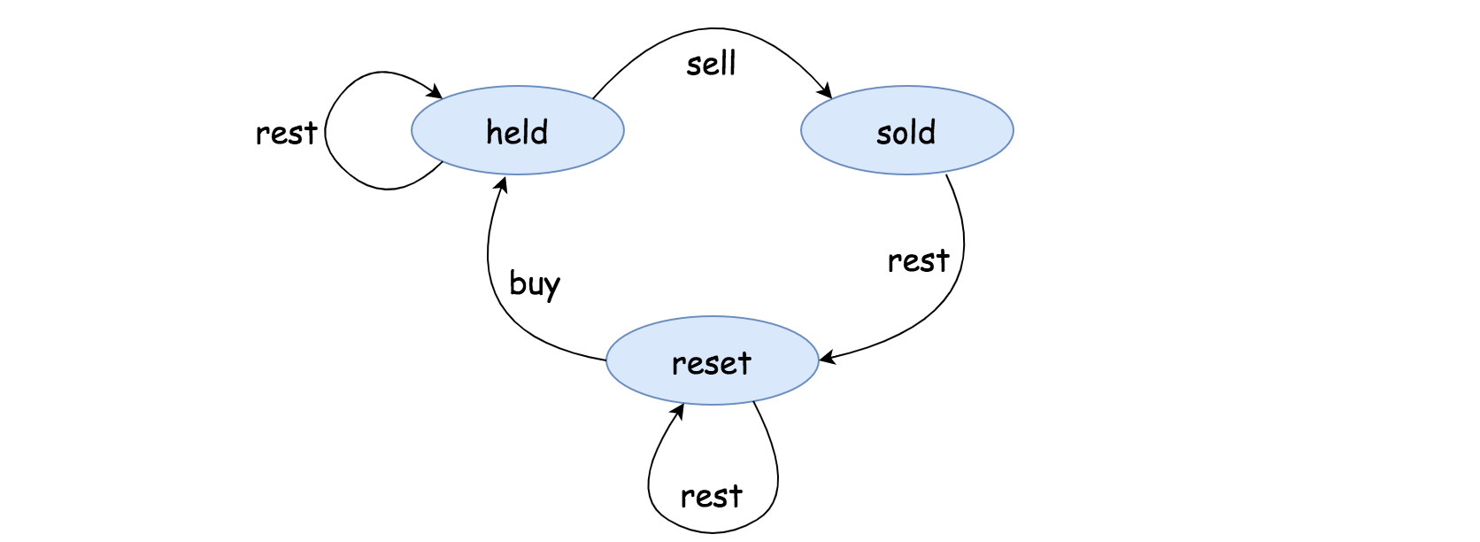
Notice that, in all states except the sold state, by doing nothing, we would remain in the same state, which is why there is a self-looped transition on these states.
Deduction
Now, one might wonder how exactly the state machine that we defined can help to solve the problem.
As we mentioned before, we model the problem as a game\, and the trader as an agent\ in the game. And this is where our state machine comes into the picture. The behaviors and the states of the game agent can be modeled by our state machine.

Given a list stock prices (i.e. price[0...n]), our agent would walk through each price point one by one. At each point, the agent would be in one of three states (i.e. held, sold and reset) that we defined before. And at each point, the agent would take one of the three actions (i.e. buy, sell and rest), which then would lead to the next state at the next price point.
Now if we chain up each state at each price point, it would form a graph\ where each path\ that starts from the initial price point and ends at the last price point represents a combination of transactions that the agent could perform through out the game.

The above graph shows all possible paths that our game agent agent walks through the list, which corresponds to all possible combinations of transactions that the trader can perform with the given price sequence.
In order to solve the problem, the goal is to find such a path in the above graph that maximizes the profits.
In each node of graph, we also indicate the maximal profits that the agent has gained so far in each state of each step. And we highlight the path that generates the maximal profits. Don’t worry about them for the moment. We will explain in detail how to calculate in the next section.
Algorithm
In order to implement the above state machine, we could define three arrays (i.e. held[i], sold[i] and reset[i]) which correspond to the three states that we defined before.
Each element in each array represents the maximal profits that we could gain at the specific price point
iwith the specific state. For instance, the elementsold[2]represents the maximal profits we gain if we sell the stock at the price pointprice[2].
According to the state machine we defined before, we can then deduce the formulas to calculate the values for the state arrays, as follows:
sold[i]=hold[i−1]+price[i]held[i]=max(held[i−1],reset[i−1]−price[i])reset[i]=max(reset[i−1],sold[i−1])sold[i]=hold[i−1]+price[i]held[i]=max(held[i−1],reset[i−1]−price[i])reset[i]=max(reset[i−1],sold[i−1])
Here is how we interpret each formulas:
- sold[i]sold[i]: the previous state of
soldcan only beheld. Therefore, the maximal profits of this state is the maximal profits of the previous state plus the revenue by selling the stock at the current price. - held[i]held[i]: the previous state of
heldcould also beheld, i.e. one does no transaction. Or its previous state could bereset, from which state, one can acquire a stock at the current price point. - reset[i]reset[i]: the previous state of
resetcould either beresetorsold. Both transitions do not involve any transaction with the stock.
Finally, the maximal profits that we can gain from this game would be max(sold[n],reset[n])max(sold[n],reset[n]), i.e. at the last price point, either we sell the stock or we simply do no transaction, to have the maximal profits. It makes no sense to acquire the stock at the last price point, which only leads to the reduction of profits.
In particular, as a base case, the game should be kicked off from the state reset, since initially we don’t hold any stock and we don’t have any stock to sell neither. Therefore, we assign the initial values of sold[-1] and held[-1] to be Integer.MIN_VALUE, which are intended to render the paths that start from these two states impossible.
As one might notice in the above formulas, in order to calculate the value for each array, we reuse the intermediate values, and this is where the paradigm of dynamic programming comes into play.
More specifically, we only need the intermediate values at exactly one step before the current step. As a result, rather than keeping all the values in the three arrays, we could use a sliding window\ of size 1 to calculate the value for max(sold[n],reset[n])max(sold[n],reset[n]).
In the following animation, we demonstrate the process on how the three arrays are calculated step by step.

1 / 7
As a byproduct\ of this algorithm, not only would we obtain the maximal profits at the end, but also we could recover each action that we should perform along the path, although this is not required by the problem.
In the above graph, by starting from the final state, and walking backward following the path, we could obtain a sequence of actions that leads to the maximal profits at the end, i.e. [buy, sell, cooldown, buy, sell].
Complexity Analysis
Time Complexity: O(N)O(N) where NN is the length of the input price list.
- We have one loop over the input list, and the operation within one iteration takes constant time.
Space Complexity: O(1)O(1), constant memory is used regardless the size of the input.
Approach 2: Yet-Another Dynamic Programming
Intuition
Most of the times, there are more than one approaches to decompose the problem, so that we could apply the technique of dynamic programming.
Here we would like to propose a different perspective on how to model the problem purely with mathematical formulas.
Again, this would be a journey loaded with mathematical notations, which might be complicated, but it showcases how the mathematics could help one with the dynamic programming (pun intended).
Definition
For a sequence of prices, denoted as price[0,1,…,n]price[0,1,…,n], let us first define our target function called MP(i)MP(i). The function MP(i)MP(i)gives the maximal profits that we can gain for the price subsequence starting from the index ii, i.e. price[i,i+1,…,n]price[i,i+1,…,n].
Given the definition of the MP(i)MP(i) function, one can see that when i=0i=0 the output of the function, i.e. MP(0)MP(0), is exactly the result that we need to solve the problem, which is the maximal profits that one can gain for the price subsequence of price[0,1,…,n]price[0,1,…,n].
Suppose that we know all the values for MP(i)MP(i) onwards until MP(n)MP(n), i.e. we know the maximal profits that we can gain for any subsequence of price[k…n]k∈[i,n]price[k…n]k∈[i,n].
Now, let us add a new price point price[i−1]price[i−1] into the subsequence price[i…n]price[i…n], all we need to do is to deduce the value for the unknown MP(i−1)MP(i−1).
Up to this point, we have just modeled the problem with our target function MP(i)MP(i), along with a series of definitions. The problem now is boiled down to deducing the formula for MP(i−1)MP(i−1).
In the following section, we will demonstrate how to deduce the formula for MP(i−1)MP(i−1).
Deduction
With the newly-added price point price[i−1]price[i−1], we need to consider all possible transactions that we can do to the stock at this price point, which can be broken down into two cases:
- Case 1): we buy this stock with price[i−1]price[i−1] and then sell it at some point in the following price sequence of price[i…n]price[i…n]. Note that, once we sell the stock at a certain point, we need to cool down for a day, then we can reengage with further transactions. Suppose that we sell the stock right after we bought it, at the next price point price[i]price[i], the maximal profits we would gain from this choice would be the profit of this transaction (i.e. price[i]−price[i−1]price[i]−price[i−1]) plus the maximal profits from the rest of the price sequence, as we show in the following:

In addition, we need to enumerate all possible points to sell this stock, and take the maximum among them. The maximal profits that we could gain from this case can be represented by the following:
C1=max{k∈[i,n]}(price[k]−p[i−1]+MP(k+2))C1=max{k∈[i,n]}(price[k]−p[i−1]+MP(k+2))
- Case 2): we simply do nothing with this stock. Then the maximal profits that we can gain from this case would be MP(i)MP(i), which are also the maximal profits that we can gain from the rest of the price sequence.
C2=MP(i)C2=MP(i)
By combining the above two cases, i.e. selecting the max value among them, we can obtain the value for MP(i−1)MP(i−1), as follows:
MP(i−1)=max(C1,C2)MP(i−1)=max(C1,C2)
MP(i−1)=max(max{k∈[i,n]}(price[k]−price[i−1]+MP(k+2)),MP(i))MP(i−1)=max(max{k∈[i,n]}(price[k]−price[i−1]+MP(k+2)),MP(i))
By the way, the base case for our recursive function MP(i)MP(i) would be MP(n)MP(n) which is the maximal profits that we can gain from the sequence with a single price point price[n]price[n]. And the best thing we should do with a single price point is to do no transaction, hence we would neither lose money nor gain any profit, i.e. MP(n)=0MP(n)=0.
The above formulas do model the problem soundly. In addition, one should be able to translate them directly into code.
Algorithm
With the final formula we derived for our target function MP(i)MP(i), we can now go ahead and translate it into any programming language.
- Since the formula deals with subsequences of price that start from the last price point, we then could do an iteration over the price list in the reversed order.
- We define an array
MP[i]to hold the values for our target function MP(i)MP(i). We initialize the array with zeros, which correspond to the base case where the minimal profits that we can gain is zero. Note that, here we did a trick to pad the array with two additional elements, which is intended to simplify the branching conditions, as one will see later. - To calculate the value for each element
MP[i], we need to look into two cases as we discussed in the previous section, namely:- Case 1). we buy the stock at the price point
price[i], then we sell it at a later point. As one might notice, the initial padding on theMP[i]array saves us from getting out of boundary in the array. - Case 2). we do no transaction with the stock at the price point
price[i].
- Case 1). we buy the stock at the price point
- At the end of each iteration, we then pick the largest value from the above two cases as the final value for
MP[i]. - At the end of the loop, the
MP[i]array will be populated. We then return the value ofMP[0], which is the desired solution for the problem.
Complexity Analysis
- Time Complexity: O(N2)O(N2) where NN is the length of the price list.
- As one can see, we have nested loops over the price list. The number of iterations in the outer loop is NN. The number of iterations in the inner loop varies from 11 to NN. Therefore, the total number of iterations that we perform is ∑i=1Ni=N⋅(N+1)2∑i=1N**i=2N⋅(N+1).
- As a result, the overall time complexity of the algorithm is O(N2)O(N2).
- Space Complexity: O(N)O(N) where NN is the length of the price list.
- We allocated an array to hold all the values for our target function MP(i)MP(i).
337. 打家劫舍 III
在上次打劫完一条街道之后和一圈房屋后,小偷又发现了一个新的可行窃的地区。这个地区只有一个入口,我们称之为“根”。 除了“根”之外,每栋房子有且只有一个“父“房子与之相连。一番侦察之后,聪明的小偷意识到“这个地方的所有房屋的排列类似于一棵二叉树”。 如果两个直接相连的房子在同一天晚上被打劫,房屋将自动报警。
计算在不触动警报的情况下,小偷一晚能够盗取的最高金额。
示例 1:
1 | 输入: [3,2,3,null,3,null,1] |
示例 2:
1 | 输入: [3,4,5,1,3,null,1] |
1 | /** |
说明
本题目本身就是动态规划的树形版本,通过此题解,可以了解一下树形问题在动态规划问题解法
我们通过三个方法不断递进解决问题
解法一通过递归实现,虽然解决了问题,但是复杂度太高
解法二通过解决方法一中的重复子问题,实现了性能的百倍提升
解法三直接省去了重复子问题,性能又提升了一步
解法一、暴力递归 - 最优子结构
在解法一和解法二中,我们使用爷爷、两个孩子、4 个孙子来说明问题
首先来定义这个问题的状态
爷爷节点获取到最大的偷取的钱数呢
首先要明确相邻的节点不能偷,也就是爷爷选择偷,儿子就不能偷了,但是孙子可以偷
二叉树只有左右两个孩子,一个爷爷最多 2 个儿子,4 个孙子
根据以上条件,我们可以得出单个节点的钱该怎么算
4 个孙子偷的钱 + 爷爷的钱 VS 两个儿子偷的钱 哪个组合钱多,就当做当前节点能偷的最大钱数。这就是动态规划里面的最优子结构
由于是二叉树,这里可以选择计算所有子节点
4 个孙子投的钱加上爷爷的钱如下
int method1 = root.val + rob(root.left.left) + rob(root.left.right) + rob(root.right.left) + rob(root.right.right)
两个儿子偷的钱如下
int method2 = rob(root.left) + rob(root.right);
挑选一个钱数多的方案则
int result = Math.max(method1, method2);
将上述方案写成代码如下
Java
public int rob(TreeNode root) {
if (root == null) return 0;
int money = root.val;
if (root.left != null) {
    money += (rob(root.left.left) + rob(root.left.right));
}

if (root.right != null) {
    money += (rob(root.right.left) + rob(root.right.right));
}

return Math.max(money, rob(root.left) + rob(root.right));
}
信心满满的提交,一次通过,然而 执行用时:837 ms,在所有 java 提交中击败了24.49%的用户 这个结果太没面子了,下个解法进行优化
解法二、记忆化 - 解决重复子问题
针对解法一种速度太慢的问题,经过分析其实现,我们发现爷爷在计算自己能偷多少钱的时候,同时计算了 4 个孙子能偷多少钱,也计算了 2 个儿子能偷多少钱。这样在儿子当爷爷时,就会产生重复计算一遍孙子节点。
于是乎我们发现了一个动态规划的关键优化点
重复子问题
我们这一步针对重复子问题进行优化,我们在做斐波那契数列时,使用的优化方案是记忆化,但是之前的问题都是使用数组解决的,把每次计算的结果都存起来,下次如果再来计算,就从缓存中取,不再计算了,这样就保证每个数字只计算一次。
由于二叉树不适合拿数组当缓存,我们这次使用哈希表来存储结果,TreeNode 当做 key,能偷的钱当做 value
解法一加上记忆化优化后代码如下:
Java
public int rob(TreeNode root) {
HashMap<TreeNode, Integer> memo = new HashMap<>();
return robInternal(root, memo);
}
public int robInternal(TreeNode root, HashMap<TreeNode, Integer> memo) {
if (root == null) return 0;
if (memo.containsKey(root)) return memo.get(root);
int money = root.val;
if (root.left != null) {
    money += (robInternal(root.left.left, memo) + robInternal(root.left.right, memo));
}
if (root.right != null) {
    money += (robInternal(root.right.left, memo) + robInternal(root.right.right, memo));
}
int result = Math.max(money, robInternal(root.left, memo) + robInternal(root.right, memo));
memo.put(root, result);
return result;
}
提交代码,执行用时:4 ms, 在所有 java 提交中击败了 54.92% 的用户,速度提高了 200 倍。太开心了。别着急,还有一个终极方案呢,连记忆化消耗的时间都省了,能省则省么。
解法三、终极解法
上面两种解法用到了孙子节点,计算爷爷节点能偷的钱还要同时去计算孙子节点投的钱,虽然有了记忆化,但是还是有性能损耗。
我们换一种办法来定义此问题
每个节点可选择偷或者不偷两种状态,根据题目意思,相连节点不能一起偷
当前节点选择偷时,那么两个孩子节点就不能选择偷了
当前节点选择不偷时,两个孩子节点只需要拿最多的钱出来就行(两个孩子节点偷不偷没关系)
我们使用一个大小为 2 的数组来表示 int[] res = new int[2] 0 代表不偷,1 代表偷
任何一个节点能偷到的最大钱的状态可以定义为
当前节点选择不偷:当前节点能偷到的最大钱数 = 左孩子能偷到的钱 + 右孩子能偷到的钱
当前节点选择偷:当前节点能偷到的最大钱数 = 左孩子选择自己不偷时能得到的钱 + 右孩子选择不偷时能得到的钱 + 当前节点的钱数
表示为公式如下
root[0] = Math.max(rob(root.left)[0], rob(root.left)[1]) + Math.max(rob(root.right)[0], rob(root.right)[1])
root[1] = rob(root.left)[0] + rob(root.right)[0] + root.val;
将公式做个变换就是代码啦
Java
public int rob(TreeNode root) {
int[] result = robInternal(root);
return Math.max(result[0], result[1]);
}
public int[] robInternal(TreeNode root) {
if (root == null) return new int[2];
int[] result = new int[2];
int[] left = robInternal(root.left);
int[] right = robInternal(root.right);

result[0] = Math.max(left[0], left[1]) + Math.max(right[0], right[1]);
result[1] = left[0] + right[0] + root.val;

return result;
}
再提交一次:
执行用时 1 ms, 在所有 java 提交中击败了 99.87% 的用户,这样的结果,我觉得可以了。
413. 等差数列划分
难度中等122收藏分享切换为英文关注反馈
如果一个数列至少有三个元素,并且任意两个相邻元素之差相同,则称该数列为等差数列。
例如,以下数列为等差数列:
1 | 1, 3, 5, 7, 9 |
以下数列不是等差数列。
1 | 1, 1, 2, 5, 7 |
数组 A 包含 N 个数,且索引从0开始。数组 A 的一个子数组划分为数组 (P, Q),P 与 Q 是整数且满足 0<=P<Q<N 。
如果满足以下条件,则称子数组(P, Q)为等差数组:
元素 A[P], A[p + 1], …, A[Q - 1], A[Q] 是等差的。并且 P + 1 < Q 。
函数要返回数组 A 中所有为等差数组的子数组个数。
示例:
1 | A = [1, 2, 3, 4] |
1 | class Solution { |
Approach #1 Brute Force [Accepted]
The most naive solution is to consider every pair of elements(with atleast 1 element between them), so that the range of elements lying between these two elements acts as a slice. Then, we can iterate over every such slice(range) to check if all the consecutive elements within this range have the same difference. For every such range found, we can increment the countcount that is used to keep a track of the required result.
Complexity Analysis
- Time complexity : O(n3)O(n3). We iterate over the range formed by every pair of elements. Here, nn refers to the number of elements in the given array AA.
- Space complexity : O(1)O(1). Constant extra space is used.
Approach #2 Better Brute Force [Accepted]
Algorithm
In the last approach, we considered every possible range and then iterated over the range to check if the difference between every consercutive element in this range is the same. We can optimize this approach to some extent, by making a small observation.
We can see, that if we are currently considering the range bound by the elements, let’s say, A[s]As and A[e]Ae, we have checked the consecutive elements in this range to have the same difference. Now, when we move on to the next range between the indices ss and e+1e+1, we again perform a check on all the elements in the range s:es:e, along with one additional pair A[e+1]A[e+1]and A[e]A[e]. We can remove this redundant check in the range s:es:e and just check the last pair to have the same difference as the one used for the previous range(same ss, incremented ee).
Note that if the last range didn’t constitute an arithmetic slice, the same elements will be a part of the updated range as well. Thus, we can omit the rest of the ranges consisting of the same starting index. The rest of the process remains the same as in the last approach.
Complexity Analysis
- Time complexity : O(n2)O(n2). Two for loops are used.
- Space complexity : O(1)O(1). Constant extra space is used.
Approach #3 Using Recursion [Accepted]
Algorithm
By making use of the observation discussed in the last approach, we know, that if a range of elements between the indices (i,j)(i,j)constitute an Arithmetic Slice, and another element A[j+1]A[j+1] is included such that A[j+1]A[j+1] and A[j]A[j] have the same difference as that of the previous common difference, the ranges between (i,j+1)(i,j+1) will constitutes an arithmetic slice. Further, if the original range (i,j)(i,j) doesn’t form an arithmetic slice, adding new elements to this range won’t do us any good. Thus, no more arithmetic slices can be obtained by adding new elements to it.
By making use of this observation, we can develop a recursive solution for the given problem as well. Assume that a sumsum variable is used to store the total number of arithmetic slices in the given array AA. We make use of a recursive function slices(A,i)which returns the number of Arithmetic Slices in the range (k,i)(k,i), but which are not a part of any range (k,j)(k,j) such that j<ij<i. It also updates sumsum with the number of arithmetic slices(total) in the current range. Thus, kk refers to the minimum index such that the range (k,i)(k,i) constitutes a valid arithmetic slice.
Now, suppose we know the number of arithmetic slices in the range (0,i−1)(0,i−1) constituted by the elements [a0,a1,a2,…a(i−1)][a0,a1,a2,…a(i−1)], to be say xx. If this range itself is an arithmetic slice, all the consecutive elements have the same difference(equal to say, a(i−1)−a(i−2)a(i−1)−a(i−2)). Now, adding a new element aia**i to it to extend the range to (0,i)(0,i) will constitute an arithmetic slice only if this new element satisfies ai−a(i−1)=a(i−1)−a(i−2)a*i−*a(i−1)=a(i−1)−a(i−2). Thus, now, the addition of this new element, will lead to an addition of apa**p number of arithmetic slices to the ones obtained in the range (0,i−1)(0,i−1). The new arithmetic slices will be the ones constituting the ranges (0,i),(1,i),…(i−2,i)(0,i),(1,i),…(i−2,i), which are a total of x+1x+1 additional arithmetic slices. This is because, apart from the range (0,i)(0,i) the rest of the ranges (1,i),(2,i),…(i−2,i)(1,i),(2,i),…(i−2,i) can be mapped to (0,i−1),(1,i−1),…(i−3,i−1)(0,i−1),(1,i−1),…(i−3,i−1), with count equal to xx.
Thus, in every call to slices, if the ithith element has the same common difference with the last element as the previous common difference, we can find the number of new arithmetic slices added by the use of this element, apa**p and also update the sumsum to include this apa**p into it, apart from the count obtained by the smaller ranges. But, if the new element doesn’t have the same common difference, extra arithmetic slices can’t be contributed by it and hence, no addition is done to sumsum for the current element. But, of course sumsum will be updated as per the count obtained from the smaller ranges.
Complexity Analysis
- Time complexity : O(n)O(n). The recursive function is called at most n−2n−2 times.
- Space complexity : O(n)O(n). The depth of the recursion tree goes upto n−2n−2.
Approach #5 Dynamic Programming [Accepted]:
Algorithm
In the last approach, we start with the full range (0,n−1)(0,n−1), where nn is the number of elements in the given AA array. We can observe that the result for the range (0,i)(0,i) only depends on the elements in the range (0,i)(0,i) and not on any element beyond this range. Thus, we can make use of Dynamic Programming to solve the given problem.
We can make use of a 1-D dpd**p with number of elements equal to nn. dp[i]d**p[i] is used to store the number of arithmetic slices possible in the range (k,i)(k,i) and not in any range (k,j)(k,j) such that j<ij<i. Again, kk refers to the minimum index possible such that (k,j)(k,j)constitutes a valid Arithmetic Slice.
Instead of going in the reverse order as in the recursive approach, we can start filling the dpd**p in a forward manner. The intuition remains the same as in the last approach. For the ithith element being considered, we check if this element satsfies the common difference criteria with the previous element. If so, we know the number of new arithmetic slices added will be 1+dp[i−1]1+d**p[i−1] as discussed in the last approach. The sumsum is also updated by the same count to reflect the new arithmetic slices added.
The following animation illustrates the dpd**p filling process.

1 / 9
Complexity Analysis
- Time complexity : O(n)O(n). We traverse over the given AA array with nn elements once only.
- Space complexity : O(n)O(n). 1-D dpd**p of size nn is used.
Approach #5 Constant Space Dynamic Programming [Accepted]:
Algorithm
In the last approach, we can observe that we only require the element dp[i−1]d**p[i−1] to determine the value to be entered at dp[i]d**p[i]. Thus, instead of making use of a 1-D array to store the required data, we can simply keep a track of just the last element.
Complexity Analysis
- Time complexity : O(n)O(n). We traverse over the given AA array with nn elements once only.
- Space complexity : O(1)O(1). Constant extra space is used.
Approach #6 Using Formula [Accepted]:
Algorithm
From the dpd**p solution, we can observe that for kk consecutive elements sastisfying the common difference criteria, we update the sumsum for each such element by 1,2,3,…,k1,2,3,…,k counts in that order. Thus, instead of updating the sumsum at the same time, we can just keep a track of the number of consecutive elements satisfying the common differnce criteria in a countcount variable and just update the sumsum directly as count∗(count+1)/2count∗(count+1)/2 whenver an element not satisfying this criteria is found. At the same time, we also need to reset the countcount value.
Complexity Analysis
- Time complexity : O(n)O(n). We iterate over AA with nn elements exactly once.
- Space complexity : O(1)O(1). Constant extra space is used.
1039. 多边形三角剖分的最低得分
难度中等41收藏分享切换为英文关注反馈
给定 N,想象一个凸 N 边多边形,其顶点按顺时针顺序依次标记为 A[0], A[i], ..., A[N-1]。
假设您将多边形剖分为 N-2 个三角形。对于每个三角形,该三角形的值是顶点标记的乘积,三角剖分的分数是进行三角剖分后所有 N-2 个三角形的值之和。
返回多边形进行三角剖分后可以得到的最低分。
示例 1:
1 | 输入:[1,2,3] |
示例 2:

1 | 输入:[3,7,4,5] |
示例 3:
1 | 输入:[1,3,1,4,1,5] |
1 | class Solution { |
解题思路
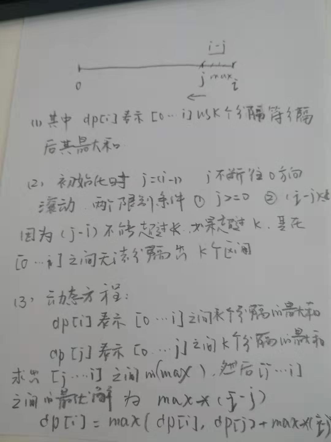
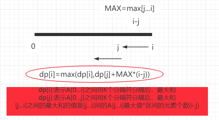
dp[i][j]表示从i到j序列的最低分。记底边为ij的三角形顶点为m,三角形imj将多边形分成三部分,总分即为三部分的分数和(如果m=i+1或m=j-1,则对应第一或第三部分分数为0)。
那么m在什么位置分数最低呢,将m从i+1到j-1遍历,分别计算dp[i][m]+A[i]A[j]A[m]+dp[m][j],取其中最小值即为dp[i][j]。
dp[i][j]=min(dp[i][m]+A[i]A[j]A[m]+dp[m][j]),for m in range [i+1,j-1]
dp table只用到右上半部分,初始化相邻两元素序列结果为0(两元素序列不能构成三角形);采用自底向上、自左向右的方向计算dp table。最终输出dp[0][n-1]。
1043. 分隔数组以得到最大和
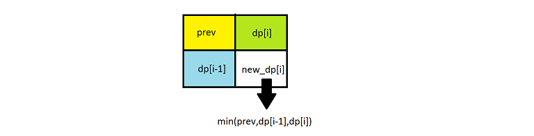
难度中等48收藏分享切换为英文关注反馈
给出整数数组 A,将该数组分隔为长度最多为 K 的几个(连续)子数组。分隔完成后,每个子数组的中的值都会变为该子数组中的最大值。
返回给定数组完成分隔后的最大和。
示例:
1 | 输入:A = [1,15,7,9,2,5,10], K = 3 |
提示:
1 <= K <= A.length <= 5000 <= A[i] <= 10^6
1 | class Solution { |
方法1:DP
1218. 最长定差子序列
难度中等27收藏分享切换为英文关注反馈
给你一个整数数组 arr 和一个整数 difference,请你找出 arr 中所有相邻元素之间的差等于给定 difference 的等差子序列,并返回其中最长的等差子序列的长度。
示例 1:
1 | 输入:arr = [1,2,3,4], difference = 1 |
示例 2:
1 | 输入:arr = [1,3,5,7], difference = 1 |
示例 3:
1 | 输入:arr = [1,5,7,8,5,3,4,2,1], difference = -2 |
提示:
1 <= arr.length <= 10^5-10^4 <= arr[i], difference <= 10^4
1 | class Solution { |
思路
这道题思路比较简单,跟经典问题最长递增(减)子序列有点相似,而这道题称为最长等差子序列, 也就是说是固定公差的递增(减),相对还更简单一点。
可以用dp[i]来记录以数字i为结尾的最长等差子序列的长度,那么它应该只有两种情况:
dp[i] = 1 // 表示在 i 之前没有出现等差子序列
dp[i] = dp[i - difference] + 1 // 表示在 i 之前出现了等差子序列,长度为 dp[i - difference], 而 i 也是满足这个等差序列的,所以等差序列的长度在此基础上加 1 就可以了
考虑元素值会出现负数,所以用数组存放是不行的,那么可以用一个 map来维护以 i 结尾的最长等差序列的长度,所以也就不难得出如下代码:
可以为下标加一个偏置,解决出现负值的情况,这是很OK,因为这道题arr[i]、difference的数据范围已经给的很明确了,而且比较小。
1269. 停在原地的方案数
难度困难23收藏分享切换为英文关注反馈
有一个长度为 arrLen 的数组,开始有一个指针在索引 0 处。
每一步操作中,你可以将指针向左或向右移动 1 步,或者停在原地(指针不能被移动到数组范围外)。
给你两个整数 steps 和 arrLen ,请你计算并返回:在恰好执行 steps 次操作以后,指针仍然指向索引 0 处的方案数。
由于答案可能会很大,请返回方案数 模 10^9 + 7 后的结果。
示例 1:
1 | 输入:steps = 3, arrLen = 2 |
示例 2:
1 | 输入:steps = 2, arrLen = 4 |
示例 3:
1 | 输入:steps = 4, arrLen = 2 |
提示:
1 <= steps <= 5001 <= arrLen <= 10^6s: steps
l:经过s步,停留的坐标
p[s][l]: 经过s步,停留在坐标l的总方案数
arrLen: 数组长度
1 | class Solution { |
动态规划解法三要素:
1、最优子结构
指针可以向左、向右、停在原地,所有最后一步可以前面的基础上往这三个方向前进,即子结构为:
p[s-1][l], p[s-1][l-1] , p[s-1][l+1]   PS: 原地、向右、向左
2、状态转移方程
p[s][l] = p[s-1][l] + p[s-1][l-1] + p[s-1][l+1]
3、边界条件
p[0][0] = 1;
p[s][l] = 0 if s < l

问题求解:
p[s][0]
arrLen


注意点:
1、 中间结果数组,注意边界条件p[s][l] = 0 if s < l  ,所以只需要定义int[steps+1][steps+1] 而不需要是int[steps+1][arrLen],不然会超出内存限制;
2、 结果是返回模 10^9 + 7 后的结果,p[s][l] = p[s-1][l] + p[s-1][l-1] + p[s-1][l+1]  状态方程是两两相加就要求mod,而不是三个求和之后再求mod,之前结果总有用例不过
就是因为三个求和之后再求的mod。
1312. 让字符串成为回文串的最少插入次数
难度困难34收藏分享切换为英文关注反馈
给你一个字符串 s ,每一次操作你都可以在字符串的任意位置插入任意字符。
请你返回让 s 成为回文串的 最少操作次数 。
「回文串」是正读和反读都相同的字符串。
示例 1:
1 | 输入:s = "zzazz" |
示例 2:
1 | 输入:s = "mbadm" |
示例 3:
1 | 输入:s = "leetcode" |
示例 4:
1 | 输入:s = "g" |
示例 5:
1 | 输入:s = "no" |
提示:
1 <= s.length <= 500s中所有字符都是小写字母。
我们用 dp[i][j] 表示对于字符串 s 的子串 s[i:j](这里的下标从 0 开始,并且 s[i:j] 包含 s 中的第 i 和第 j 个字符),最少添加的字符数量,使得 s[i:j] 变为回文串。
我们从外向内考虑 s[i:j]:
如果 s[i] == s[j],那么最外层已经形成了回文,我们只需要继续考虑 s[i+1:j-1];
如果 s[i] != s[j],那么我们要么在 s[i:j] 的末尾添加字符 s[i],要么在 s[i:j] 的开头添加字符 s[j],才能使得最外层形成回文。如果我们选择前者,那么需要继续考虑 s[i+1:j];如果我们选择后者,那么需要继续考虑 s[i:j-1]。
因此我们可以得到如下的状态转移方程:
dp[i][j] = min(dp[i + 1][j] + 1, dp[i][j - 1] + 1) if s[i] != s[j]
dp[i][j] = min(dp[i + 1][j] + 1, dp[i][j - 1] + 1, dp[i + 1][j - 1]) if s[i] == s[j]
边界条件为:
dp[i][j] = 0 if i >= j
注意该动态规划为区间动态规划,需要注意 dp[i][j] 的计算顺序。一种可行的方法是,我们递增地枚举子串 s[i:j] 的长度 span = j - i + 1,再枚举起始位置 i,通过 j = i + span - 1 得到 j 的值并计算 dp[i][j]。这样的计算顺序可以保证在计算 dp[i][j] 时,状态转移方程中的状态 dp[i + 1][j],dp[i][j - 1] 和 dp[i + 1][j - 1] 均已计算过。
1 | class Solution { |
509. 斐波那契数
难度简单118收藏分享切换为英文关注反馈
斐波那契数,通常用 F(n) 表示,形成的序列称为斐波那契数列。该数列由 0 和 1 开始,后面的每一项数字都是前面两项数字的和。也就是:
1 | F(0) = 0, F(1) = 1 |
给定 N,计算 F(N)。
示例 1:
1 | 输入:2 |
示例 2:
1 | 输入:3 |
示例 3:
1 | 输入:4 |
提示:
- 0 ≤
N≤ 30
1 | class Solution { |
Approach 1: Recursion
Intuition
Use recursion to compute the Fibonacci number of a given integer.

Figure 1. An example tree representing what fib(5) would look like
Algorithm
- Check if the provided input value, N, is less than or equal to 1. If true, return N.
- Otherwise, the function
fib(int N)calls itself, with the result of the 2 previous numbers being added to each other, passed in as the argument. This is derived directly from therecurrence relation: Fn=Fn−1+Fn−2F**n=F*n−1+F*n−2 - Do this until all numbers have been computed, then return the resulting answer.
Complexity Analysis
- Time complexity : O(2N)O(2N). This is the slowest way to solve the
Fibonacci Sequencebecause it takes exponential time. The amount of operations needed, for each level of recursion, grows exponentially as the depth approachesN. - Space complexity : O(N)O(N). We need space proportionate to
Nto account for the max size of the stack, in memory. This stack keeps track of the function calls tofib(N). This has the potential to be bad in cases that there isn’t enough physical memory to handle the increasingly growing stack, leading to aStackOverflowError. The Java docs have a good explanation of this, describing it as an error that occurs because an application recurses too deeply.
Approach 2: Bottom-Up Approach using Memoization
Intuition
Improve upon the recursive option by using iteration, still solving for all of the sub-problems and returning the answer for N, using already computed Fibonacci values. In using a bottom-up approach, we can iteratively compute and store the values, only returning once we reach the result.
Algorithm
- If
Nis less than or equal to 1, returnN - Otherwise, iterate through
N, storing each computed answer in an array along the way. - Use this array as a reference to the 2 previous numbers to calculate the current Fibonacci number.
- Once we’ve reached the last number, return it’s Fibonacci number.
Complexity Analysis
- Time complexity : O(N)O(N). Each number, starting at 2 up to and including
N, is visited, computed and then stored for O(1)O(1)access later on. - Space complexity : O(N)O(N). The size of the data structure is proportionate to
N.
Approach 3: Top-Down Approach using Memoization
Intuition
Solve for all of the sub-problems, use memoization to store the pre-computed answers, then return the answer for N. We will leverage recursion, but in a smarter way by not repeating the work to calculate existing values.
Algorithm
- Check if
N <= 1. If it is, returnN. - Call and return
memoize(N) - If
Nexists in the map, return the cached value forN - Otherwise set the value of
N, in our mapping, to the value ofmemoize(N-1) + memoize(N-2)
Complexity Analysis
- Time complexity : O(N)O(N). Each number, starting at 2 up to and including
N, is visited, computed and then stored for O(1)O(1)access later on. - Space complexity : O(N)O(N). The size of the stack in memory is proportionate to
N.
Approach 4: Iterative Top-Down Approach
Intuition
Let’s get rid of the need to use all of that space and instead use the minimum amount of space required. We can achieve O(1)O(1)space complexity by only storing the value of the two previous numbers and updating them as we iterate to N.
Algorithm
- Check if
N <= 1, if it is then we should returnN. - Check if
N == 2, if it is then we should return1sinceNis 2 andfib(2-1) + fib(2-2)equals1 + 0 = 1. - To use an iterative approach, we need at least 3 variables to store each state
fib(N),fib(N-1)andfib(N-2). - Preset the initial values:
- Initialize
currentwith 0. - Initialize
prev1with 1, since this will representfib(N-1)when computing the current value. - Initialize
prev2with 1, since this will representfib(N-2)when computing the current value.
- Initialize
- Iterate, incrementally by 1, all the way up to and including
N. Starting at 3, since0,1and2are pre-computed. - Set the
currentvalue tofib(N-1) + fib(N-2)because that is the value we are currently computing. - Set the
prev2value tofib(N-1). - Set the
prev1value tocurrent_value. - When we reach
N+1, we will exit the loop and return the previously setcurrentvalue.
Complexity Analysis
- Time complexity : O(N)O(N). Each value from
2 to Nwill be visited at least once. The time it takes to do this is directly proportionate toNwhereNis theFibonacci Numberwe are looking to compute. - Space complexity : O(1)O(1). This requires 1 unit of Space for the integer
Nand 3 units of Space to store the computed values (curr,prev1andprev2) for every loop iteration. The amount of Space doesn’t change so this is constant Space complexity.
Approach 5: Matrix Exponentiation
Intuition
Use Matrix Exponentiation to get the Fibonacci number from the element at (0, 0) in the resultant matrix.
In order to do this we can rely on the matrix equation for the Fibonacci sequence, to find the Nth Fibonacci number: (1 11 0)n=( F(n+1) F(n) F(n) F(n−1))(1110)n=(F(n+1)F(n)F(n)F(n−1))
Algorithm
- Check if
Nis less than or equal to 1. If it is, returnN. - Use a recursive function,
matrixPower, to calculate the power of a given matrixA. The power will beN-1, whereNis theNth Fibonacci number. - The
matrixPowerfunction will be performed forN/2of the Fibonacci numbers. - Within
matrixPower, call themultiplyfunction to multiply 2 matrices. - Once we finish doing the calculations, return
A[0][0]to get theNthFibonacci number.
Complexity Analysis
- Time complexity : O(logN)O(logN). By halving the
Nvalue in everymatrixPower‘s call to itself, we are halving the work needed to be done. - Space complexity : O(logN)O(logN). The size of the stack in memory is proportionate to the function calls to
matrixPowerplus the memory used to account for the matrices which takes up constant space.
Approach 6: Math
Intuition Using the golden ratio, a.k.a Binet's forumula: φ=1+52≈1.6180339887….φ=21+5≈1.6180339887….
Here’s a link to find out more about how the Fibonacci sequence and the golden ratio work.
We can derive the most efficient solution to this problem using only constant time and constant space!
Algorithm
- Use the
golden ratioformula to calculate theNthFibonacci number.
Complexity Analysis
- Time complexity : O(1)O(1). Constant time complexity since we are using no loops or recursion and the time is based on the result of performing the calculation using
Binet's formula. - Space complexity : O(1)O(1). The space used is the space needed to create the variable to store the
golden ratioformula.
面试题 17.16. 按摩师
难度简单98收藏分享切换为英文关注反馈
一个有名的按摩师会收到源源不断的预约请求,每个预约都可以选择接或不接。在每次预约服务之间要有休息时间,因此她不能接受相邻的预约。给定一个预约请求序列,替按摩师找到最优的预约集合(总预约时间最长),返回总的分钟数。
注意:本题相对原题稍作改动
示例 1:
1 | 输入: [1,2,3,1] |
示例 2:
1 | 输入: [2,7,9,3,1] |
示例 3:
1 | 输入: [2,1,4,5,3,1,1,3] |
1 | class Solution { |
《程序员面试金典(第 6 版)》独家授权![]()

本书是原谷歌资深面试官的经验之作,帮助了许多想要加入脸书、苹果、谷歌等 IT 名企的求职者拿到 Dream offer。本专题的 100+ 编程面试题是在原书基础上精心挑选出来的,帮助你轻松应战 IT 名企技术面试。