94. 二叉树的中序遍历
难度中等477收藏分享切换为英文关注反馈
给定一个二叉树,返回它的中序 遍历。
示例:
1 | 输入: [1,null,2,3] |
进阶: 递归算法很简单,你可以通过迭代算法完成吗?
1 | /** |
1 | /** |
102. 二叉树的层序遍历
难度中等454收藏分享切换为英文关注反馈
给你一个二叉树,请你返回其按 层序遍历 得到的节点值。 (即逐层地,从左到右访问所有节点)。
示例:
二叉树:[3,9,20,null,null,15,7],
1 | 3 |
返回其层次遍历结果:
1 | [ |
1 | /** |
1 | /** |
103. 二叉树的锯齿形层次遍历
难度中等183收藏分享切换为英文关注反馈
给定一个二叉树,返回其节点值的锯齿形层次遍历。(即先从左往右,再从右往左进行下一层遍历,以此类推,层与层之间交替进行)。
例如:
给定二叉树 [3,9,20,null,null,15,7],
1 | 3 |
返回锯齿形层次遍历如下:
1 | [ |
1 | /** |
Approach 1: BFS (Breadth-First Search)
Intuition
Following the description of the problem, the most intuitive solution would be the BFS (Breadth-First Search) approach through which we traverse the tree level-by-level.
The default ordering of BFS within a single level is from left to right. As a result, we should adjust the BFS algorithm a bit to generate the desired zigzag ordering.
One of the keys here is to store the values that are of the same level with the
deque(double-ended queue) data structure, where we could add new values on either end of a queue.
So if we want to have the ordering of FIFO (first-in-first-out), we simply append the new elements to the tail of the queue, i.e. the late comers stand last in the queue. While if we want to have the ordering of FILO (first-in-last-out), we insert the new elements to the head of the queue, i.e. the late comers jump the queue.

Algorithm
There are several ways to implement the BFS algorithm.
- One way would be that we run a two-level nested loop, with the outer loop iterating each level on the tree, and with the inner loop iterating each node within a single level.
- We could also implement BFS with a single loop though. The trick is that we append the nodes to be visited into a queue and we separate nodes of different levels with a sort of delimiter (e.g. an empty node). The delimiter marks the end of a level, as well as the beginning of a new level.
Here we adopt the second approach above. One can start with the normal BFS algorithm, upon which we add a touch of zigzag*order with the help of deque. For each level, we start from an empty deque container to hold all the values of the same level. Depending on the ordering of each level, *i.e. either from-left-to-right or from-right-to-left, we decide at which end of the deque to add the new element:

- For the ordering of from-left-to-right (FIFO), we append the new element to the tail\ of the queue, so that the element that comes late would get out late as well. As we can see from the above graph, given an input sequence of
[1, 2, 3, 4, 5], with FIFO ordering, we would have an output sequence of[1, 2, 3, 4, 5]. - For the ordering of from-right-to-left (FILO), we insert the new element to the head\ of the queue, so that the element that comes late would get out first. With the same input sequence of
[1, 2, 3, 4, 5], with FILO ordering, we would obtain an output sequence of[5, 4, 3, 2, 1].
Note: as an alternative approach, one can also implement the normal BFS algorithm first, which would generate the ordering of from-left-to-right for each of the levels. Then, at the end of the algorithm, we can simply reverse\ the ordering of certain levels, following the zigzag steps.
Complexity Analysis
Time Complexity: O(N)O(N), where NN is the number of nodes in the tree.
- We visit each node once and only once.
- In addition, the insertion operation on either end of the deque takes a constant time, rather than using the array/list data structure where the inserting at the head could take the O(K)O(K) time where KK is the length of the list.
Space Complexity: O(N)O(N) where NN is the number of nodes in the tree.
The main memory consumption of the algorithm is the
node_queuethat we use for the loop, apart from the array that we use to keep the final output.As one can see, at any given moment, the
node_queuewould hold the nodes that are at most across two levels. Therefore, at most, the size of the queue would be no more than 2⋅L2⋅L, assuming LL is the maximum number of nodes that might reside on the same level. Since we have a binary tree, the level that contains the most nodes could occur to consist all the leave nodes in a full binary tree, which is roughly L=N2L=2N. As a result, we have the space complexity of 2⋅N2=N2⋅2N=N in the worst case.
Approach 2: DFS (Depth-First Search)
Intuition
Though not intuitive, we could also obtain the BFS traversal ordering via the DFS (Depth-First Search) traversal in the tree.
The trick is that during the DFS traversal, we maintain the results in a global array that is indexed by the level, i.e. the element
array[level]would contain all the nodes that are at the same level. The global array would then be referred and updated at each step of DFS.

Similar with the above modified BFS algorithm, we employ the deque data structure to hold the nodes that are of the same level, and we alternate the insertion direction (i.e. either to the head or to the tail) to generate the desired output ordering.
Algorithm
Here we implement the DFS algorithm via recursion. We define a recursive function called DFS(node, level) which only takes care of the current node which is located at the specified level. Within the function, here are three steps that we would perform:
- If this is the first time that we visit any node at the
level, i.e. the deque for the level does not exist, then we simply create the deque with the current node value as the initial element. - If the deque for this level exists, then depending on the ordering, we insert the current node value either to the head or to the tail of the queue.
- At the end, we recursively call the function for each of its child nodes.
It might go without saying that, one can also implement the DFS traversal via iteration\ rather than recursion, which could be one of the followup questions by an interviewer.
Complexity Analysis
- Time Complexity: O(N)O(N), where NN is the number of nodes in the tree.
- Same as the previous BFS approach, we visit each node once and only once.
- Space Complexity: O(H)O(H), where HH is the height of the tree, i.e. the number of levels in the tree, which would be roughly log2Nlog2N.
- Unlike the BFS approach, in the DFS approach, we do not need to maintain the
node_queuedata structure for the traversal. - However, the function recursion would incur additional memory consumption on the function call stack. As we can see, the size of the call stack for any invocation of
DFS(node, level)would be exactly the number oflevelthat the current node resides on. Therefore, the space complexity of our DFS algorithm is O(log2N)O(log2N) which is much better than the BFS approach.
- Unlike the BFS approach, in the DFS approach, we do not need to maintain the
107. 二叉树的层次遍历 II
难度简单235收藏分享切换为英文关注反馈
给定一个二叉树,返回其节点值自底向上的层次遍历。 (即按从叶子节点所在层到根节点所在的层,逐层从左向右遍历)
例如:
给定二叉树 [3,9,20,null,null,15,7],
1 | 3 |
返回其自底向上的层次遍历为:
1 | [ |
1 | class Solution { |
How to traverse the tree
There are two general strategies to traverse a tree:
Depth First Search (
DFS)In this strategy, we adopt the
depthas the priority, so that one would start from a root and reach all the way down to a certain leaf, and then back to root to reach another branch.The DFS strategy can further be distinguished as
preorder,inorder, andpostorderdepending on the relative order among the root node, left node, and right node.Breadth First Search (
BFS)We scan through the tree level by level, following the order of height, from top to bottom. The nodes on a higher level would be visited before the ones on lower levels.
In the following figure the nodes are enumerated in the order you visit them, please follow 1-2-3-4-5 to compare different strategies.

Here the problem is to implement split-level BFS traversal : [[4, 5], [2, 3], [1]]. That means we could use one of the Node->Left->Right techniques: BFS or DFS Preorder.
We already discussed three different ways to implement iterative BFS traversal with the queue, and compared iterative BFS vs. iterative DFS. Let’s use this article to discuss the two most simple and fast techniques:
- Recursive DFS.
- Iterative BFS with two queues.
Note, that both approaches are root-to-bottom traversals, and we’re asked to provide bottom-up output. To achieve that, the final result should be reversed.
Approach 1: Recursion: DFS Preorder Traversal
Intuition
The first step is to ensure that the tree is not empty. The second step is to implement the recursive function helper(node, level), which takes the current node and its level as the arguments.
Algorithm for the Recursive Function
Here is its implementation:
- Initialize the output list
levels. The length of this list determines which level is currently updated. You should compare this levellen(levels)with a node levellevel, to ensure that you add the node on the correct level. If you’re still on the previous level - add the new level by adding a new list intolevels. - Append the node value to the last level in
levels. - Process recursively child nodes if they are not
None:helper(node.left / node.right, level + 1).
Implementation

1 / 16
Complexity Analysis
Time complexity: O(N)O(N) since each node is processed exactly once.
Space complexity: O(N)O(N) to keep the output structure which contains NN node values.
Approach 2: Iteration: BFS Traversal
Algorithm
The recursion above could be rewritten in the iteration form.
Let’s keep each tree level in the queue structure, which typically orders elements in a FIFO (first-in-first-out) manner. In Java one could use ArrayDeque implementation of the Queue interface. In Python using Queue structure would be an overkill since it’s designed for a safe exchange between multiple threads and hence requires locking which leads to a performance downgrade. In Python the queue implementation with a fast atomic append() and popleft() is deque.
Algorithm
- Initialize two queues: one for the current level, and one for the next. Add root into
nextLevelqueue. - While
nextLevelqueue is not empty:- Initialize the current level
currLevel = nextLevel, and empty the next levelnextLevel. - Iterate over the current level queue:
- Append the node value to the last level in
levels. - Add first left and then right child node into
nextLevelqueue.
- Append the node value to the last level in
- Initialize the current level
- Return reversed
levels.
Implementation
Complexity Analysis
- Time complexity: O(N)O(N) since each node is processed exactly once.
- Space complexity: O(N)O(N) to keep the output structure which contains NN node values.
230. 二叉搜索树中第K小的元素
难度中等216收藏分享切换为英文关注反馈
给定一个二叉搜索树,编写一个函数 kthSmallest 来查找其中第 k 个最小的元素。
说明:
你可以假设 k 总是有效的,1 ≤ k ≤ 二叉搜索树元素个数。
示例 1:
1 | 输入: root = [3,1,4,null,2], k = 1 |
示例 2:
1 | 输入: root = [5,3,6,2,4,null,null,1], k = 3 |
进阶:
如果二叉搜索树经常被修改(插入/删除操作)并且你需要频繁地查找第 k 小的值,你将如何优化 kthSmallest 函数?
1 | //recursion |
How to traverse the tree
There are two general strategies to traverse a tree:
Depth First Search (
DFS)In this strategy, we adopt the
depthas the priority, so that one would start from a root and reach all the way down to certain leaf, and then back to root to reach another branch.The DFS strategy can further be distinguished as
preorder,inorder, andpostorderdepending on the relative order among the root node, left node and right node.Breadth First Search (
BFS)We scan through the tree level by level, following the order of height, from top to bottom. The nodes on higher level would be visited before the ones with lower levels.
On the following figure the nodes are numerated in the order you visit them, please follow 1-2-3-4-5 to compare different strategies.

To solve the problem, one could use the property of BST : inorder traversal of BST is an array sorted in the ascending order.
Approach 1: Recursion
It’s a very straightforward approach with O(N)O(N) time complexity. The idea is to build an inorder traversal of BST which is an array sorted in the ascending order. Now the answer is the k - 1th element of this array.

Complexity Analysis
Time complexity : O(N)O(N) to build a traversal.
Space complexity : O(N)O(N) to keep an inorder traversal.
Approach 2: Iteration
The above recursion could be converted into iteration, with the help of stack. This way one could speed up the solution because there is no need to build the entire inorder traversal, and one could stop after the kth element.

Complexity Analysis
Time complexity : O(H+k)O(H+k), where HH is a tree height. This complexity is defined by the stack, which contains at least H+kH+k elements, since before starting to pop out one has to go down to a leaf. This results in O(logN+k)O(logN+k) for the balanced tree and O(N+k)O(N+k) for completely unbalanced tree with all the nodes in the left subtree.
Space complexity : O(H+k)O(H+k), the same as for time complexity, O(N+k)O(N+k) in the worst case, and O(logN+k)O(logN+k) in the average case.
Follow up
What if the BST is modified (insert/delete operations) often and you need to find the kth smallest frequently? How would you optimize the kthSmallest routine?
Insert and delete in a BST were discussed last week, the time complexity of these operations is O(H)O(H), where HH is a height of binary tree, and H=logNH=logN for the balanced tree.
Hence without any optimisation insert/delete + search of kth element has O(2H+k)O(2H+k) complexity. How to optimise that?
That’s a design question, basically we’re asked to implement a structure which contains a BST inside and optimises the following operations :
- Insert
- Delete
- Find kth smallest
Seems like a database description, isn’t it? Let’s use here the same logic as for LRU cache design, and combine an indexing structure (we could keep BST here) with a double linked list.
Such a structure would provide:
- O(H)O(H) time for the insert and delete.
- O(k)O(k) for the search of kth smallest.

The overall time complexity for insert/delete + search of kth smallest is O(H+k)O(H+k) instead of O(2H+k)O(2H+k).
Complexity Analysis
- Time complexity for insert/delete + search of kth smallest: O(H+k)O(H+k), where HH is a tree height. O(logN+k)O(logN+k) in the average case, O(N+k)O(N+k) in the worst case.
- Space complexity : O(N)O(N) to keep the linked list.
501. 二叉搜索树中的众数
难度简单109收藏分享切换为英文关注反馈
给定一个有相同值的二叉搜索树(BST),找出 BST 中的所有众数(出现频率最高的元素)。
假定 BST 有如下定义:
- 结点左子树中所含结点的值小于等于当前结点的值
- 结点右子树中所含结点的值大于等于当前结点的值
- 左子树和右子树都是二叉搜索树
例如:
给定 BST [1,null,2,2],
1 | 1 |
返回[2].
提示:如果众数超过1个,不需考虑输出顺序
进阶:你可以不使用额外的空间吗?(假设由递归产生的隐式调用栈的开销不被计算在内)
1 | /** |
使用List即时存放出现最多的数
private List<Integer> items;
private int maxCount;
private int curCount;
private TreeNode pre;

public int[] findMode(TreeNode root) {
    if (root == null)
        return new int[0];
    items = new ArrayList<>();
    // 这里设置为1是因为 在递归中 BST中最左边的结点被跳过了,作为初状态 该结点值出现一次,记录的出现最多次数一开始也为1
    maxCount = 1;
    curCount = 1;
    midTraversal(root);
    // 最右端结点的处理,从递归中看,最后一个结点与前一个结点相等只更新了curCount的值;不相等则只考虑到倒数第二个结点。
    if(curCount > maxCount)
        return new int[]{pre.val};
    if(curCount == maxCount)
        items.add(pre.val);
    int[] res = new int[items.size()];
    for (int i = 0; i < res.length; i++)
        res[i] = items.get(i);
    return res;
}

private void midTraversal(TreeNode x) {
    if (x == null) return;
    midTraversal(x.left);
    if(pre != null){
        if(x.val != pre.val){ // 说明上一个值的结点数量已经统计完成 要看出现次数的情况
            if(curCount > maxCount){ // 出现次数更多,清空之前的出现少的数,更新最大出现次数
                maxCount = curCount;
                items.clear();
                items.add(pre.val);
            }
            else if(curCount == maxCount){ // 不止一个众数
                items.add(pre.val);
            }
            curCount = 1; // 当前值与上一个结点值不同,重置计数
        }
        else curCount++; // 当前值与上一个结点值相同,当前值的出现次数增加。
    }
    pre = x;
    midTraversal(x.right);
}
思路分析:
找众数,说明要统计出现次数,一般会直接想到搞个哈希表来计数(就像后面的方法二)。但是如果一个有序数组中统计出现次数,使用双指针就能很好解决,类似的这里给我们的树不是一般的树,而是BST,中序遍历相当于遍历有序数组。
利用BST这个特性,我们不需要使用哈希表来计数。如同双指针的做法,这里也需要记录上一个结点TreeNode pre;这样才能知道当前结点值与谁比较;另外还需要记录某个值的出现次数curCount,以及出现次数的最大值maxCount(否则你咋知道谁出现最多次)。并且这里遍历过程中的众数信息需要记录(List存放众数)及更新。
在中序遍历中:
如果pre == null,说明这是遍历的第一个结点,不需要处理(第一个结点的初条件在主函数中设定)。
如果当前结点值与上一个结点值相等,那么这个数字的出现次数+1。
否则,我们先去判断,上一个数字的出现次数curCount与之前的最大出现次数maxCount谁更大:
如果上一个数字出现次数最大,需要更新众数信息。首先更新最大出现次数maxCount = curCount;。然后将之前记录的众数清空,再将上一个数字放入items.clear(); items.add(pre.val);
如果一个数字出现次数等于最大出现次数,那么目前来看,它也是可能的众数,加入列表items.add(pre.val);
否则,上一个数字一定不是众数,不管它,继续保留List中的数字。
最后,重置计数curCount = 1;,表示当前数字出现一次了。
然后更新pre = x;
回到主函数:
特殊情况处理,root == null直接返回new int[0]。
然后上文提到的初始化,因为最左边结点在中序的递归中不处理,所以,我们要首先将maxCount = 1,因为树非空总会有数字出现一次,然后curCount = 1,代表最左边结点被我们在主函数计数了。
调用辅助函数后,还需要处理最后一个结点的值,因为在递归中不会有再下一个结点值与之不相等然后来判断它的值是否为众数。
所以如果curCount > maxCount,说明最后一个结点才是唯一众数,return new int[]{pre.val};
如果curCount == maxCount,说明最后一个结点也是众数,items.add(pre.val);
最后,将List转成数组返回。
这个题要注意边界的考虑!
时间复杂度为
O
(
n
)
O(n), 不考虑递归调用栈的话,空间复杂度可以认为是常数,中间状态List的元素并不会很多。
543. 二叉树的直径
难度简单372收藏分享切换为英文关注反馈
给定一棵二叉树,你需要计算它的直径长度。一棵二叉树的直径长度是任意两个结点路径长度中的最大值。这条路径可能穿过也可能不穿过根结点。
示例 :
给定二叉树
1 | 1 |
返回 3, 它的长度是路径 [4,2,1,3] 或者 [5,2,1,3]。
1 | class Solution { |
Approach #1: Depth-First Search [Accepted]
Intuition
Any path can be written as two arrows (in different directions) from some node, where an arrow is a path that starts at some node and only travels down to child nodes.
If we knew the maximum length arrows L, R for each child, then the best path touches L + R + 1 nodes.
Algorithm
Let’s calculate the depth of a node in the usual way: max(depth of node.left, depth of node.right) + 1. While we do, a path “through” this node uses 1 + (depth of node.left) + (depth of node.right) nodes. Let’s search each node and remember the highest number of nodes used in some path. The desired length is 1 minus this number.
Complexity Analysis
- Time Complexity: O(N)O(N). We visit every node once.
- Space Complexity: O(N)O(N), the size of our implicit call stack during our depth-first search.
663. Equal Tree Partition
Given a binary tree with n nodes, your task is to check if it’s possible to partition the tree to two trees which have the equal sum of values after removing exactly one edge on the original tree.
Example 1:
1 | Input: |
Example 2:
1 | Input: |
Note:
- The range of tree node value is in the range of [-100000, 100000].
- 1 <= n <= 10000
1 | class Solution { |
Approach #1: Depth-First Search [Accepted]
Intuition and Algorithm
After removing some edge from parent to child, (where the child cannot be the original root) the subtree rooted at child must be half the sum of the entire tree.
Let’s record the sum of every subtree. We can do this recursively using depth-first search. After, we should check that half the sum of the entire tree occurs somewhere in our recording (and not from the total of the entire tree.)
Our careful treatment and analysis above prevented errors in the case of these trees:
1 | 0 |
Complexity Analysis
- Time Complexity: O(N)O(N) where NN is the number of nodes in the input tree. We traverse every node.
- Space Complexity: O(N)O(N), the size of
seenand the implicit call stack in our DFS.
1339. 分裂二叉树的最大乘积
难度中等26收藏分享切换为英文关注反馈
给你一棵二叉树,它的根为 root 。请你删除 1 条边,使二叉树分裂成两棵子树,且它们子树和的乘积尽可能大。
由于答案可能会很大,请你将结果对 10^9 + 7 取模后再返回。
示例 1:
1 | 输入:root = [1,2,3,4,5,6] |
示例 2:
1 | 输入:root = [1,null,2,3,4,null,null,5,6] |
示例 3:
1 | 输入:root = [2,3,9,10,7,8,6,5,4,11,1] |
示例 4:
1 | 输入:root = [1,1] |
提示:
- 每棵树最多有
50000个节点,且至少有2个节点。 - 每个节点的值在
[1, 10000]之间。
1 | class Solution { |
Approach 1: One-Pass DFS
Intuition
To get started, we’re just going to pretend that integers can be infinitely large.
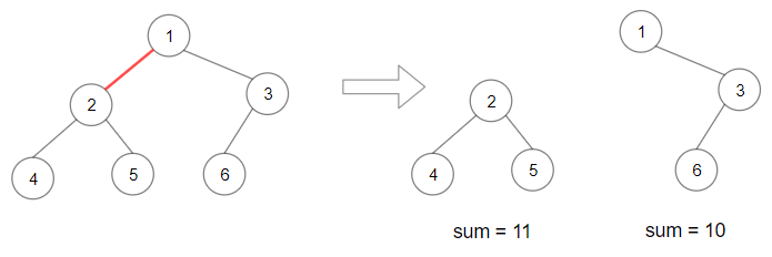
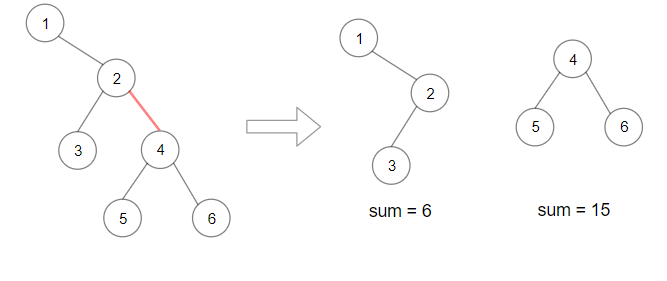
We’ll use the following tree example.

There are n - 1 edges in a tree with n nodes, and so for this question there are n - 1 different possible ways of splitting the tree into a pair of subtrees. Here are 4 out of the 10 possible ways.

Of these 4 possible ways, the best is the third one, which has a product of 651.
To make it easier to discuss the solution, we’ll name each of the subtrees in a pair.
- One of the new subtrees is rooted at the node below the removed edge. We’ll call it
Subtree 1. - The other is rooted at the root node of the original tree, and is missing the subtree below the removed edge. We’ll call it
Subtree 2.

Remember that we’re required to find the pair of subtrees that have the maximum product. This is done by calculating the sum of each subtree and then multiplying them together. The sum of a subtree is the sum of all the nodes in it.
Calculating the sum of Subtree 1 can be done using the following recursive tree algorithm. The root of Subtree 1 is passed into the function.
1 | def tree_sum(subroot): |
This algorithm calculates the sum of a subtree by calculating the sum of its left subtree, sum of its right subtree, and then adding these to the root value. The sum of the left and right subtrees is done in the same way by the recursion.

If you’re confused by this recursive summing algorithm, it might help you to read this article on solving tree problems with recursive (top down) algorithms.
We still need a way to calculate the sum of Subtree 2. Recall that Subtree 2 is the tree we get by removing Subtree 1. The only way we could directly use the above summing algorithm to calculate the sum of Subtree 2 is to actually remove the edge above Subtree 1 first. Otherwise, Subtree 1 would be automatically traversed too.
A simpler way is to recognise that Sum(Subtree 2) = Sum(Entire Tree) - Sum(Sub Tree 1).

Another benefit of this approach is that we only need to calculate Sum(Entire Tree) once. Then, for each Sum(Subtree 1) we calculate, we can immediately calculate Sum(Subtree 2) as an O(1)O(1) operation.
Recall how the summing algorithm above worked. The recursive function is called once for every node in the tree (i.e. subtree rooted at that node), and returns the sum of that subtree.

Therefore we can simply gather up all the possible Subtree 1 sums with a list as follows:
1 | subtree_1_sums = [] # All Subtree 1 sums will go here. |
Now that we have a list of the sums for all possible Subtree 1‘s, we can calculate what the corresponding Subtree 2 would be for each of them, and then calculate the product, keeping track of the best seen so far.
1 | # Call the function. |
The question also says we need to take the answer modulo 10 ^ 9 + 7. Expanded out, this number is 1,000,000,007. So when we return the product, we’ll do:
1 | best_product % 1000000007 |
Only take the final product modulo 10 ^ 9 + 7. Otherwise, you might not be correctly comparing the products.
Up until now, we’ve assumed that integers can be of an infinite size. This is a safe assumption for Python, but not for Java. For Java (and other languages that use a 32-bit integer by default), we’ll need to think carefully about where integer overflows could occur.
The problem statement states that there can be up to 50000 nodes, each with a value of up to 10000. Therefore, the maximum possible subtree sum would be 50,000 * 10,000 = 500,000,000. This is well below the size of a 32-bit integer (2,147,483,647). Therefore, it is impossible for an integer overflow to occur during the summing phase with these constraints.
However, multiplying the subtrees could be a problem. For example, if we had subtrees of 100,000,000 and 400,000,000, then we’d get a total product of 400,000,000,000,000,000 which is definitely larger than a 32-bit integer, and therefore and overflow would occur!
The easiest solution is to instead use 64-bit integers. In Java, this is the long primitive type. The largest possible product would be 250,000,000 * 250,000,000 = 62,500,000,000,000,000, which is below the maximum a 64-bit integer can hold.
In Approach #3, we discuss other ways of solving the problem if you only had access to 32-bit integers.
Algorithm
Complexity Analysis
nn is the number of nodes in the tree.
Time Complexity : O(n)O(n).
The recursive function visits each of the nn nodes in the tree exactly once, performing an O(1)O(1) recursive operation on each. This gives a total of O(n)O(n)
There are n−1n−1 numbers in the list. Each of these is processed with an O(1)O(1) operation, giving a total of O(n)O(n) time for this phase too.
In total, we have O(n)O(n).
Space Complexity O(n)O(n).
There are two places that extra space is used.
Firstly, the recursion is putting frames on the stack. The maximum number of frames at any one time is the maximum depth of the tree. For a balanced tree, this is around O(log n)O(logn), and in the worst case (a long skinny tree) it is O(n)O(n).
Secondly, the list takes up space. It contains n−1n−1 numbers at the end, so it too is O(n)O(n).
In both the average case and worst case, we have a total of O(n)O(n) space used by this approach.
Something you might have realised is that the subtree pair that leads to the largest product is the pair with the smallest difference between them. Interestingly, this fact doesn’t help us much with optimizing the algorithm. This is because subtree sums are notobtained in sorted order, and so any attempt to sort them (and thus find the nearest to middle directly) will cost at least O(n log n)O(nlogn) to do. With the overall algorithm, even with the linear search, only being O(n)O(n), this is strictly worse. The only situation this insight becomes useful is if you have to solve the problem using only 32-bit integers. The reason for this is discussed in Approach #3.
Approach 2: Two-Pass DFS
Intuition
Instead of putting the Subtree 1 sums into a separate list, we can do 2 separate tree summing traversals.
- Calculate the sum of the entire tree.
- Check the product we’d get for each subtree.
Calculating the total sum is done in the same way as before.
Finding the maximum product is similar, except requires a variable outside of the function to keep track of the maximum product seen so far.
1 | def maximum_product(subroot, total): |
Algorithm
It is possible to combine the 2 recursive functions into a single one that is called twice, however the side effects of the functions (changing of class variables) hurt code readability and can be confusing. For this reason, the code below uses 2 separate functions.
Complexity Analysis
nn is the number of nodes in the tree.
Time Complexity : O(n)O(n).
Each recursive function visits each of the nn nodes in the tree exactly once, performing an O(1)O(1) recursive operation on each. This gives a total of O(n)O(n).
Space Complexity O(n)O(n).
The recursion is putting frames on the stack. The maximum number of frames at any one time is the maximum depth of the tree. For a balanced tree, this is around O(log n)O(logn), and in the worst case (a long skinny tree) it is O(n)O(n).
Because we use worst case for complexity analysis, we say this algorithm uses O(n)O(n) space. However, it’s worth noting that as long as the tree is fairly balanced, the space usage will be a lot nearer to O(log n)O(logn).
Approach 3: Advanced Strategies for Dealing with 32-Bit Integers
Intuition
This is an advanced bonus section that discusses ways of solving the problem using only 32-bit integers. It’s not essential for an interview, although could be useful depending on your choice of programming language. Some of the ideas might also help with potential follow up questions. This section assumes prior experience with introductory modular arithmetic.
We’ll additionally assume that the 32-bit integer we’re working with is signed, so has a maximum value of 2,147,483,647.
What if your chosen programming language only supported 32-bit integers, and you had no access to a Big Integer library? Could we still solve this problem? What are the problems we’d need to address?
The solutions above relied on being able to multiply 2 numbers of up to 30 (signed) bits each without overflow. Because the number of bits in the product add, we would expect the product to require ~60 bits to represent. Using a 64-bit integer was therefore enough. Additionally, with a modulus of 1,000,000,007, the final product, after taken to the modulus, will always fit within a 32-bit integer.
However, we’re now assuming that we only have 32-bit integers. When working with 32-bit integers, we must always keep the total below 2,147,483,647, even during intermediate calculations. Therefore, we’ll need a way of doing the math within this restriction. One way to do the multiplication safely is to write an algorithm using the same underlying idea as modular exponentiation.
1 | private int modularMultiplication(int a, int b, int m) { |
There is one possible pitfall with this though. We are supposed to return the calculation for the largest product, determined before the modulus is taken.
For example, consider the following 2 products:
34,000 * 30,000 = 1,020,000,000becomes1,020,000,000 % 1,000,000,007 = 19,999,993.30,000 * 30,000 = 900,000,000doesn’t change because900,000,000 % 1,000,000,007 = 900,000,000.
So if we were to compare them before taking the modulus, product 1 would be larger, which is correct. But if we compared them after, then product 2 is larger, which is incorrect.
Therefore, we need a way to determine which product will be the biggest, without actually calculating them. Then once we know which is biggest, we can use our method for calculating a product modulo 1,000,000,007 without going over 2,147,483,647.
The trick is to realise that Sum(Subtree 1) + Sum(Subtree 2) is constant, but Sum(Subtree 1) * Sum(Subtree 2) increases as Sum(Subtree 1) - Sum(Subtree 2) gets nearer to 0, i.e. as the sum of the subtrees is more balanced. A good way of visualising this is to imagine you have X meters of fence and need to make a rectangular enclosure for some sheep. You want to maximise the area. It turns out that the optimal solution is to make a square. The nearer to a square the enclosure is, the nearer to the optimal area it will be. For example, where H + W = 11, the best (integer) solution is 5 x 6 = 30.

A simple way to do this in code is to loop over the list of all the sums and find the (sum, total - sum) pair that has the minimal difference. This approach ensures we do not need to use floating point numbers.
Algorithm
We’ll use Approach #1 as a basis for the code, as it’s simpler and easier to understand. The same ideas can be used in Approach #2 though.
Complexity Analysis
nn is the number of nodes in the tree.
Time Complexity : O(n)O(n).
Same as above approaches.
Space Complexity : O(n)O(n).
Same as above approaches.
The modularMultiplication function has a time complexity of O(log b)O(logb) because the loop removes one bit from bb each iteration, until there are none left. This doesn’t bring up the total time complexity to O(n log b)O(nlogb) though, because bb has a fixed upper limit of 32, and is therefore treated as a constant.